Open Sourcing Farm Card Calculations

Overview

1. Project Background
2. What are ‘farm cards’?
3. Setting Up
4. Getting Data
5. Processing
6. Questions?

Background

When I started at Kendall County, “farm” and “cards” were not words I used in the same sentence. I had no idea what they were. But someone told me they were my job responsibility, so I had to figure it out!

Fortunately, my predecessor left decent notes, and our program had good documentation, so I was able to muddle through. But it left me with the distinct sense that things could, and should, be better.

What We Had

• Proprietary
• Expensive
• Dependent upon 2 additional proprietary softwares (ArcMap and MS Access)
• Used deprecated file types
• Time consuming
• Inaccurate!

We’re talking about assessments, that is, people’s taxes. If it’s not accurate, that is real money people are over or under paying! Someone is getting cheated out of their money.

We happened to be have an accompanying software for our assessments that would blindly overwrite parcel details using the output of this tool, and it was revealed that this was causing acreage values to drift year over year.

For one thing, certain tax exemptions have hard acreage cutoffs, so even a small difference can be expensive. For another, the altered values were being put back into the same tool with each successive year, in some cases leading to acreage values changing by substantial amounts.

What I Wanted

• Accurate
• Simple
• Fast
• Accessible

We tried a few different approaches.

• Model Builder in ArcGIS Pro / QGIS
• ArcGIS Python API
• PostGIS query

But eventually we settled on Python, and in particular, GeoPandas. I’m happy to say, it has accomplished all my goals.

What are Farm Cards?

TLDR

It’s how we generate property values for agricultural parcels. Values are derived from a parcel’s slope, soil type, and land use.

Full details can be found in the Illinois Department of Revenue’s Publication 122.

This makes sense. An acre of flat silt loam in cultivation is worth more than an acre of sandy hillside with a barn on it.

It’s important to point out here that actually reading Publication 122 was critical in developing a good process. The old method we had came with its own instructions, but it was purpose built for importing into our assessments database. There was nothing in the instuctions to actually explain why the various steps were being performed.

By referring back to Publication 122, we could tailor our process to meeting the requirements of the state, not simply those of a software vendor.

Individual Soil Weighting Method

There is a 10-step process given for how these calculations are done. Our primary focus has been step four:

Determine the acreage of each soil type within each land use category that will be assessed by productivity.

In other words, a spatial overlay.

Steps 1 through 3 are data management: keeping landuse, parcels, and soils up to date. We do this throughout the year between GIS and Assessments. Steps 5 through 10 are math: applying various calculations based on the values derived in step 4. This is handled by our Assessments software.

Set up the Environment

Modules

import geopandas as gp
import pandas as pd
import numpy as np

import requests
import matplotlib.pyplot as plt
import os
from pathlib import Path
from datetime import datetime

Globals

sr = "{'wkid': 3435}"

parcels_url = 'https://maps.co.kendall.il.us/server/rest/services/Hosted/Current_Cadastral_Features/FeatureServer/1/query?'
soils_url   = 'https://maps.co.kendall.il.us/server/rest/services/Hosted/Assessor_Soils/FeatureServer/0/query?'
landuse_url = 'https://maps.co.kendall.il.us/server/rest/services/Hosted/Assessor_Landuse/FeatureServer/0/query?'

out_dir = os.path.expanduser('~/')
export_name = f"farms_{datetime.now().strftime('%Y%m%d-%H%M')}"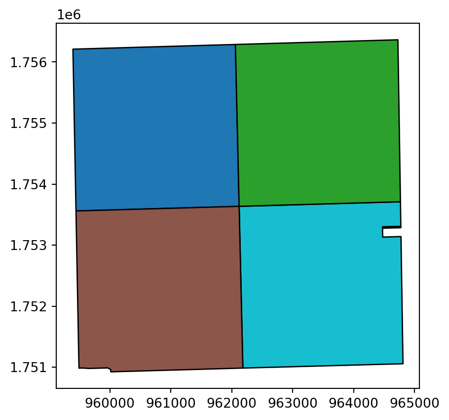
file = os.path.join(out_dir, f'{export_name}.txt')

Spatial reference, layer URLs, file handling.

Getting Data: Parcels

parcels_params = {
    'where': "pin_dashless LIKE '0827%' and class IN ('0011', '0021')",
    'outFields': 'gross_acres, pin',
    'outSR': sr,
    'f': 'geojson'
}

parcels = requests.get(parcels_url, parcels_params)
p_df = gp.read_file(parcels.text)

p_df.sample()

	pin	gross_acres	geometry
0	08-27-400-008	158.85	POLYGON ((964473.520 1753276.450, 964473.180 1...

Kendall County manages their layers in an ArcGIS Feature Service, so we couldn’t avoid at least touching a proprietary system, but I wanted to make sure that this process at least was as open and inter-operable as possible. That in mind, I chose to use requests to get features from the server.

Other Data Sources?

GeoPandas can handle pretty much anything, thanks to the Fiona module.

• Shapefiles (zipped and unzipped)
• File Geodatabases
• GeoPackages
• GeoJSON
• PostGIS
• Other spatial database tables (with some help from Pandas)

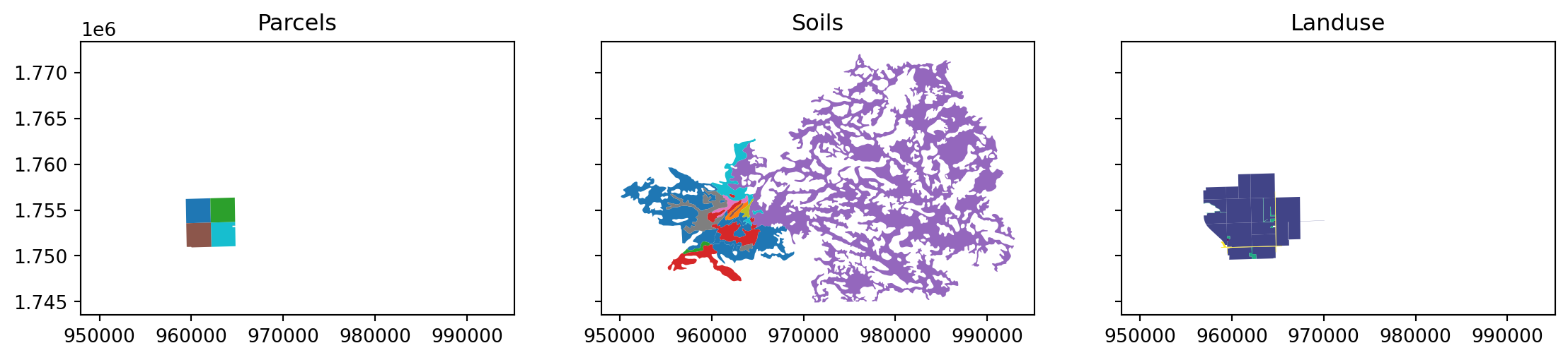
Getting Data: Soil and Landuse

Create a Spatial Filter

We’ll use the bounding box of our parcels to query any features that intersect with the parcels.

print(p_df.total_bounds)

bbox = ','.join([str(i) for i in p_df.total_bounds])
print(bbox)

[ 959392.83004983 1750923.23637091  964808.8100315  1756364.02995124]
959392.8300498277,1750923.2363709062,964808.810031496,1756364.0299512371

farm_params = {
    'where': '1=1',
    'outFields': '*',
    'returnGeometry': True,
    'geometryType': 'esriGeometryEnvelope',
    'geometry': bbox,
    'spatialRel': 'esriSpatialRelIntersects',
    'outSR': sr,
    'f': 'geojson'
}

soils = requests.get(soils_url, farm_params)
s_df = gp.read_file(soils.text)
s_df.loc[:, 'slope'].fillna('', inplace=True)

landuse = requests.get(landuse_url, farm_params)
l_df = gp.read_file(landuse.text)

We do a quick fillna on the soils layer, because certain soil types like “W” (water) have no slope code, and that can mess up the aggregation later on.

Visualize Layers

Calculated Area

Deeded acres ≠ Measured acres

We need a ratio

\[ \frac{DeedAc_{part}}{DeedAc_{whole}} = \frac{MeasFt^{2}_{part}}{MeasFt^{2}_{whole}} \\ \big\downarrow \\ DeedAc_{part} = DeedAc_{whole} * \frac{MeasFt^{2}_{part}}{MeasFt^{2}_{whole}} \]

The difference is usually pretty small, but not always. A farm parcel that hasn’t changed since the 1800s might have a legal acreage of 40, but a measured acreage several acres larger or smaller.

Add Area to Parcels

p_df['calc_area'] = p_df.area
p_df.sample()

	pin	gross_acres	geometry	calc_area
2	08-27-100-001	160.0199	POLYGON ((962120.200 1753635.080, 962059.160 1...	7.089146e+06

Data Manipulation

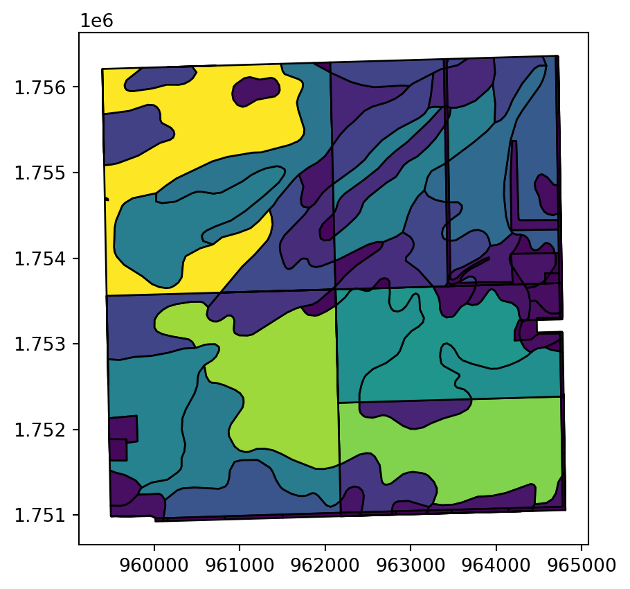
Spatial Overlay

df = gp.overlay(p_df, s_df, how='intersection')
df = gp.overlay(df, l_df, how='intersection')

df.sample(2)

	pin	gross_acres	calc_area	soil_type	muname	globalid_1	musym	slope	SHAPE__Length_1	objectid_1	...	created_user	landuse	globalid_2	landuse_type	last_edited_date	created_date	SHAPE__Length_2	objectid_2	SHAPE__Area_2	geometry
73	08-27-100-001	160.0199	7.089146e+06	330	Peotone silty clay loam, 0 to 2 percent slopes	{B91AB7B3-0048-4DF2-8EA3-3C7E9AF4FAA2}	330A	A1	1.164396e+04	5727	...	jcarlson	CR	{5BB53B1C-6DE7-4437-80CA-66D27165C57D}	2	1689080298000	1689080298000	19494.803128	2523	6.524488e+06	POLYGON ((962081.614 1755311.678, 962061.878 1...
138	08-27-200-001	160.0503	7.052477e+06	235	Bryce silty clay, 0 to 2 percent slopes	{06C67944-4F22-4A6D-9075-4D765B3CCECC}	235A	A1	1.058461e+06	4851	...	jcarlson	ROW	{D055454D-64CD-49D2-A11F-3F77D8B37343}	6	1689080298000	1689080298000	1387.146435	71669	1.990635e+04	POLYGON ((964735.912 1755700.543, 964735.912 1...

2 rows × 22 columns

Remove Extra Fields

keepers = [
    'gross_acres',
    'gis_acres',
    'calc_area',
    'pin',
    'soil_type',
    'slope',
    'landuse_type',
    'geometry'
]

df.drop(columns=[c for c in df if c not in keepers], inplace=True)

df.sample()

	pin	gross_acres	calc_area	soil_type	slope	landuse_type	geometry
141	08-27-400-008	158.85	6.948153e+06	44	A1	6	POLYGON ((963479.829 1751019.891, 963479.829 1...

Calculating Part Area

df['part_acres'] = df.area / df['calc_area'] * df['gross_acres']

df.plot(
    column='part_acres',
    edgecolor="black"
)

Validate Results

Check Acreage Sums

qc = df.groupby('pin').agg({'gross_acres':'max', 'part_acres':'sum'}).reset_index()
qc['diff'] = qc['gross_acres'] - round(qc['part_acres'], 4)

qc.sort_values(by='diff', ascending=False).head()

	pin	gross_acres	part_acres	diff
0	08-27-100-001	160.0199	160.0199	0.0
1	08-27-200-001	160.0503	160.0503	0.0
2	08-27-300-002	162.5298	162.5298	0.0
3	08-27-400-007	0.1800	0.1800	0.0
4	08-27-400-008	158.8500	158.8500	0.0

A reminder here: everything so far has just been math. So if we see a discrepancy here, it’s got to be due to errors in the data layers themselves.

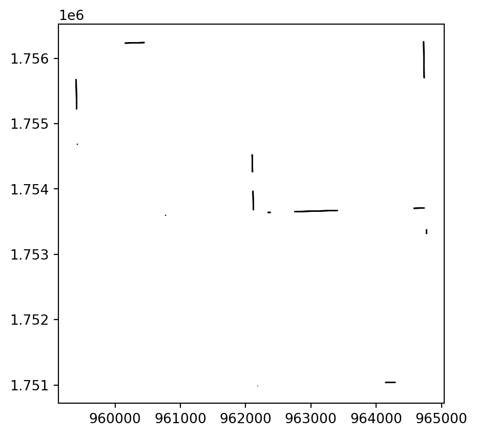
Visualize Gaps

diff_df = p_df.overlay(
    l_df,
    'symmetric_difference'
)

diff_df.plot(
    column='pin',
    edgecolor='black'
)

By using a symmetric difference overlay, we get the areas where only one of our layers had features.

Tidy Up and Export

Fields

df.drop(columns=['gross_acres', 'calc_area', 'geometry'], inplace=True)

df.loc[:,'pin'] = df['pin'].str.replace('-', '')
df.loc[:, 'landuse_type'] = '0' + df['landuse_type'].astype('str')

df.sample()

	pin	soil_type	slope	landuse_type	part_acres
14	0827100001	44	A1	02	3.629458e-07

We don’t need those calculation fields for the export file, now that we have the part_acres.

The database we’re importing into needs the hyphens stripped out of our parcel numbers, and stores landuse codes as strings with leading zeroes. 🙄

Agregating

out_cols = ['pin', 'soil_type', 'slope', 'landuse_type']

aggs = {
    'soil_type':'first',
    'slope':'first',
    'landuse_type':'first',
    'pin':'first',
    'part_acres':'sum'
}

agg_df = df.groupby(by=out_cols, as_index=False).agg(aggs).reset_index(drop=True)

agg_df.head()

	soil_type	slope	landuse_type	pin	part_acres
0	101	A1	02	0827100001	0.019314
1	137	A1	02	0827100001	30.233261
2	137	B1	02	0827100001	7.898314
3	152	A1	02	0827100001	30.680595
4	324	B1	02	0827100001	0.821661

Our overlays returned singlepart geometries, so the dataframe may have rows in which the only difference is the acreage. For valuation, we just need to total acreage per soil/landuse/slope combination, so we can aggregate those values.

It’s not strictly necessary, but makes for a more concise output.

Rounding and Filtering

agg_df.sort_values(by='part_acres').head()

	soil_type	slope	landuse_type	pin	part_acres
55	235	A1	01	0827400008	2.485521e-07
48	137	A1	04	0827400008	2.818391e-06
61	69	A1	04	0827400008	1.106778e-02
7	44	A1	04	0827100001	1.594348e-02
43	189	A1	06	0827400007	1.796944e-02

agg_df.loc[:, 'part_acres'] = round(agg_df.loc[:, 'part_acres'], 4)

agg_df = agg_df[agg_df.loc[:, 'part_acres'] > 0]

Anything beyond 4 decimal places is too precise for our assessment database. Our overlays can create tiny features, which, when imported, round off to 0.0000 acres. These rows can be dropped from the output entirely.

Export to File

0   101 A1  02  0827100001  0.0193
1   137 A1  02  0827100001  30.2333
2   137 B1  02  0827100001  7.8983
3   152 A1  02  0827100001  30.6806
4   324 B1  02  0827100001  0.8217
5   330 A1  02  0827100001  25.2632
6   44  A1  02  0827100001  64.817
7   44  A1  04  0827100001  0.0159
8   69  A1  02  0827100001  0.2706
9   101 A1  02  0827200001  8.4191
10  137 A1  02  0827200001  15.7057
11  137 A1  04  0827200001  0.7579
12  137 B1  02  0827200001  27.1341
13  137 B1  04  0827200001  0.3285
14  152 A1  02  0827200001  12.5491
15  189 A1  01  0827200001  0.0617
16  189 A1  02  0827200001  1.2277
17  189 A1  04  0827200001  3.366
18  235 A1  01  0827200001  0.3729
19  235 A1  02  0827200001  18.0763
20  235 A1  04  0827200001  3.2155
21  235 A1  06  0827200001  1.5946
22  324 B1  02  0827200001  8.5981
23  324 B1  04  0827200001  0.1339
24  325 B1  02  0827200001  7.2118
25  325 B1  04  0827200001  0.3255
26  330 A1  02  0827200001  6.8945
27  67  A1  02  0827200001  22.261
28  67  A1  04  0827200001  0.4837
29  69  A1  02  0827200001  17.9257
30  69  A1  04  0827200001  1.1287
31  91  A1  02  0827200001  2.0659
32  91  A1  06  0827200001  0.2125
33  101 A1  02  0827300002  28.0172
34  137 A1  01  0827300002  1.1427
35  137 A1  02  0827300002  55.2876
36  137 A1  04  0827300002  2.0482
37  137 A1  06  0827300002  1.7998
38  149 A1  02  0827300002  2.4657
39  152 A1  02  0827300002  58.2811
40  152 A1  06  0827300002  0.1124
41  44  A1  02  0827300002  13.3751
42  189 A1  02  0827400007  0.162
43  189 A1  06  0827400007  0.018
44  101 A1  02  0827400008  50.6161
45  101 A1  04  0827400008  0.2853
46  101 A1  06  0827400008  0.3412
47  137 A1  02  0827400008  6.2651
49  137 A1  06  0827400008  1.3067
50  152 A1  02  0827400008  84.5602
51  152 A1  06  0827400008  0.9759
52  189 A1  02  0827400008  2.4665
53  189 A1  04  0827400008  1.0565
54  189 A1  06  0827400008  0.101
56  235 A1  02  0827400008  2.267
57  235 A1  06  0827400008  0.2318
58  44  A1  02  0827400008  4.0168
59  44  A1  06  0827400008  1.1258
60  69  A1  02  0827400008  3.2228
61  69  A1  04  0827400008  0.0111

For Kendall County, this is the finish line. In spite of its name, Pandas’ to_csv() method can write to any file type we like.

Valuation

Sure, for me the process is over. But I’m not content to tell someone “just trust me” when the numbers are feeding into a black box.

But the process is openly documented, and we have the numbers. So why not do the valuation portion anyway? While I cannot actually dictate what software the County uses, I can at least validate their numbers for some peace of mind.

Extra Tables

• Soil Productivity Index Values
• Slope and Erosion Adjustment Coefficients
• Equalized Assessed Value / PI Table

pi_df = pd.read_csv(Path('soil_PI.csv').resolve())
pi_df.sample(5)

	map_symbol	soil_type	favorability	productivity_index
596	692	Beasley silt loam	Favorable	95.0
719	841	Carmi - Westland complex	Favorable	99.0
858	977	Neotoma-Wellston complex	Unfavorable	74.0
472	556	High Gap loam	Unfavorable	84.0
704	824	Schuline silt loam	Favorable	82.0

se_df = pd.read_csv(Path('soil_slope_erosion.csv').resolve())
se_df.sample(5)

	erosion_code	slope_desc	eros_desc	coeff_fav	coeff_unf
7	B3	2-5%	SEVERE	0.86	0.76
2	A2	0-2%	MODERATE	0.96	0.93
22	F2	18-35%	MODERATE	0.72	0.69
26	G2	35-70%	MODERATE	0.42	0.37
10	C2	5-10%	MODERATE	0.92	0.88

Slope and Erosion Coefficients

Our soil data comes with slope / erosion codes with the following ranges:

Code	%Slope
None / A	00 - 02
B	02 - 05
C	05 - 10
D	10 - 15
E	15 - 18
F	18 - 35
G	35 - 70

Per Pub 122:

Because Table 3 cannot be used with slope ranges, use a central point of the slope ranges unless a better determinant of slope is available.

EAV

Table 1 in Pub 122 gives us the per-acre EAV for a given PI.

However! There is a minimum certified PI.

To calculate values below that minimum, IDOR provides the following calculations, and we take whichever is greater.

\[ EAV^{PI_{n}} = EAV^{PI_{min}} - \left(\frac{EAV^{PI_{min+5}} - EAV^{PI_{min}}}{5} * (min - n)\right) \]

\[ EAV^{PI_{n}} = \frac{EAV^{PI_{min}}}{3} \]

eav_df = pd.read_csv(Path('eav_2022.csv').resolve())

sub82 = pd.DataFrame({'avg_PI': np.arange(1,82)})
sub82['eav'] = 199.29 - (((207.47-199.29)/5)*(82-sub82['avg_PI']))

print(f'Floor: {199.29/3:0.5}')
eav = pd.concat([eav_df, sub82])
eav.sort_values(by='avg_PI').head(3)

Floor: 66.43

	avg_PI	eav
0	1	66.774
1	2	68.410
2	3	70.046

We’ve got the 2022 numbers in here, so we’re just hard-coding the calculation. Note the Floor we print out. Even a PI of 1 is still higher than this, so the calculated values will always be greater than the simple division.

Merge DataFrames

val_df = agg_df.merge(pi_df, how='left', left_on='soil_type', right_on='map_symbol', suffixes=('','_desc'))
val_df = val_df.merge(se_df, how='left', left_on='slope', right_on='erosion_code')

val_df.sample(2)

	soil_type	slope	landuse_type	pin	part_acres	map_symbol	soil_type_desc	favorability	productivity_index	erosion_code	slope_desc	eros_desc	coeff_fav	coeff_unf
48	137	A1	06	0827400008	1.3067	137	Clare silt loam, bedrock substratum	Favorable	113.0	A1	0-2%	UNERODED	1.0	1.0
30	69	A1	04	0827200001	1.1287	69	Milford silty clay loam	Favorable	113.0	A1	0-2%	UNERODED	1.0	1.0

Adjusted PI

val_df.insert(
    5,
    'adj_PI',
    np.where(
        val_df['favorability'] == 'Favorable',
        val_df['productivity_index'] * val_df['coeff_fav'],
        val_df['productivity_index'] * val_df['coeff_unf']
    )
)

val_df[['productivity_index', 'favorability', 'adj_PI']].sample(3)

	productivity_index	favorability	adj_PI
48	113.0	Favorable	113.0
54	107.0	Favorable	107.0
15	115.0	Favorable	115.0

Here we use the favorability and associated coefficients to derive the adjusted PI.

Merge in EAVs

val_df.loc[:,'adj_PI'] = val_df.loc[:,'adj_PI'].round()
val_df = val_df.merge(eav_df, how='left', left_on='adj_PI', right_on='avg_PI')

val_df[['landuse_type', 'avg_PI', 'eav']].sample(4)

	landuse_type	avg_PI	eav
44	02	111	426.08
13	04	112	436.56
50	06	127	807.19
19	02	107	394.41

We round off our PI here, because the EAV values are based on PI integers.

Landuse Adjustments

Landuse	Calculation
Cropland	\(EAV\)
Permanent Pasture	\(\frac{EAV}{3}\)
Other Farmland	\(\frac{EAV}{6}\)
Contributory Wasteland	\(33.22\)

For the big three, it’s the EAV itself, or divided by something. Contributory wasteland gets a flat rate. Everything else is 0.

val_df.insert(6, 'eav_adj', 0)

val_df.loc[val_df['landuse_type'] == '02', 'eav_adj'] = val_df['eav'] 
val_df.loc[val_df['landuse_type'] == '03', 'eav_adj'] = val_df['eav']/3
val_df.loc[val_df['landuse_type'] == '04', 'eav_adj'] = val_df['eav']/6
val_df.loc[val_df['landuse_type'] == '05', 'eav_adj'] = 33.22

val_df[['landuse_type', 'eav', 'eav_adj']].sample(5)

	landuse_type	eav	eav_adj
0	02	426.08	426.08
32	06	369.43	0.00
27	02	491.66	491.66
2	02	436.56	436.56
42	02	469.07	469.07

Multiply EAV by Acres

val_df['value'] = val_df['part_acres'] * val_df['eav_adj']

val_df[['pin', 'soil_type', 'slope', 'landuse_type', 'part_acres', 'value']].fillna(0).sample(5)

	pin	soil_type	slope	landuse_type	part_acres	value
49	0827400008	152	A1	02	84.5602	68256.147838
52	0827400008	189	A1	04	1.0565	82.595409
10	0827200001	137	A1	02	15.7057	7023.903154
28	0827200001	67	A1	04	0.4837	39.635990
0	0827100001	101	A1	02	0.0193	8.223344

That’s the farm card!

Per-Parcel Totals

	part_acres	value
pin
0827100001	160.0199	73548.277557
0827200001	160.0504	68556.261183
0827300002	162.5298	89997.880404
0827400007	0.1800	75.989340
0827400008	158.8498	97539.361467

And how does this compare?

PIN	Mine	Theirs
0827100001	73,548.28	73,550.00
0827200001	68,556.26	68,550.00
0827300002	89,997.88	90,000.00
0827400005	52,400.21	52,400.00
0827400006	45,154.87	45,150.00
0827400007	75.99	80.00

There’s some rounding going on, but my numbers are consistent with the way the current tool crunches the numbers. So at least we now know we can trust those numbers, provided the input comes in okay.

Taking Things Further

• Standalone function that takes lists / input files of parcel numbers
• Wrap process in a GUI for other staff
• Put function into cloud environment, trigger via API?
• Generate per-parcel PDFs w/ maps, tables

Questions?

Be in Touch!

josh@jcarlson.page

https://jcarlson.page

@jcarlson@mapstodon.space